In This Article
Audio Filters & Equalization
An audio equalizer is a device developed throughout the past century to affect the amplitude of select frequencies. The type of equalizer you choose will determine how you affect your signal, and with the options in today’s market they can seem endless. Starting out as an audio engineer or producer in 2023, there are no shortage of tools and plugins that you can utilize in your productions, and one of the most common would undoubtedly be an equalizer [EQ]. Depending on the size of your project, you might even use several different EQs multiple times throughout your session, each one with a different purpose in mind. In some cases, you’re fixing a problem resonance and the next you’re adjusting the tonal balance with a boost or cut over large swaths of frequencies. But, how are you sure of the affect it has on your signal? Of course you’re using your ears to determine the difference, but why might one equalizer sound different than another?
With that question in mind, the aim of this article is to take a more or less agnostic approach to the process of equalization. I will discuss briefly the historical context that has brought us to this point, as it felt prudent to illustrate some pivotal innovations that ultimately brought us to today’s use cases. The end goal here being for you to understand the general concept of audio filtration and equalization to better equip yourself while mixing.
From understanding the components of early hardware equalizers, we’ll move on to the evolution of digital computation and the advantages, as well as limitations we face with modern EQs. [A quick disclaimer: I am not an electrical engineer. I have however, through the years of using these tools and learning about their history, formed a familiarity with the material enough to hopefully display these concepts clearly to a lay reader.]
Throughout this article I will be using common terminology used while describing audio equalizers (as well as in the discussion of audio engineering at large). Some of these innovations can be traced back to the late 1800s / early 1900s, with related terminology having their derivation attributed to the many advancements in engineering and transmission lines. The language hasn’t evolved too much since and can dissuade new audio engineers and producers looking to enter the field. I found it helpful to understand how and when these innovations were initially implemented, to give some context for later advancements — although I will try to limit the history lesson. The focus of these next few sections is to be able to understand the components, parameters, and concepts surrounding audio equalizers [both analog and digital], and feel confident in your decision making when reaching to use one.
Below are a few terms that will be used in the next section. You may skip ahead if you are already familiar with these terms within the context of audio equalization.
Bandwidth - When referring to a set range of frequencies within your signal, one might refer to it as a bandwidth. You may hear the terms “lows,” “mids,” and “highs,” when referring to general audible ranges of frequencies. While these bandwidths are slightly nebulous in regards to their separation, we’ll try to take a more exacting approach when delineating the frequencies or bandwidths we aim to affect.
Resonance - A resonance with regard to digital audio is a spike in amplitude within your signal. In acoustic pressure, a resonance may occur from a sound wave propagating within a space and causing a particular frequency to resonate within said space. Depending on the room mode, (more or less the dimensions of the room that causes certain frequencies to have a slight “bump” in amplitude) this resonance can be attenuated during the recording process.
Equalization - This process was originally intended to effectively reduce problem resonances in amplitude, roughly equalizing the signal across the auditory bandwidth. With modern advances in technology, equalization has become a much more creative method of accentuating your signal — offering both the option to boost or cut select bandwidths of individual channels within your mix.
What is a Filter?
I think a good place to start is by defining what a filter is and how it pertains to an equalizer. In terms of audio signal processing, a filter is generally described as a device that attenuates at specific frequencies or limits the bandwidth of the overall signal. You can think of your ears as filters that limit your perception of audio frequencies between 20Hz and 20kHz (the general bandwidth for human hearing). There are a number of filter types that we will go into detail on further down, but in general these circuits were created to “equalize” the signal to resemble as close to its original transmission as possible. You may have heard the terms “boost” or “cut” to increase or decrease your signal, or perhaps the fancier term “attenuate” when aiming to reduce a particular frequency. It is important to know what scale you’re working within, to better understand how you’re affecting your signal. You’re likely familiar with the term “decibel,” or dB when referring to how loud something in the near vicinity might be. A decibel (or 0.1 bel) is a unit that expresses the logarithmic ratio between two physical quantities, which can refer to voltage, electrical currents, or acoustic pressure waves. This term was coined after Alexander Graham Bell, the inventor of the telephone and responsible for the eventual formation of a company you may have heard of, AT&T.
While you don’t need to know the math involved in these processes to utilize audio equipment or software, it’s beneficial to understand this reference scale in regards to signal processing. In most DAWs (Digital Audio Workstations), the default readout would be in dBfs or decibels full scale, which is used for amplitude levels in digital systems. You may have also heard of dBV for measuring voltage, dbSPL for sound pressure level, and still there are more depending on the units and physical quantities you are measuring. In the process of equalization you are generally using a filter to modify the signal by altering the amplitude of frequencies present. In the analog domain this process takes place through the particular sequence of electrical components to reduce or increase the gain level of a targeted bandwidth of frequencies. Now at this point, If you are an “in-the-box” producer / engineer working primarily with software plugins, you might be wondering why any of this information about the “analog” domain is pertinent or useful. I should remind you that you are in fact using speakers and headphones to listen to your signal though, and those require some amount of audio filtration to accurately reproduce the signal’s playback from within your DAW.
Passive vs. Active filters
Audio filters have been advanced numerous times before reaching their current form today, starting out as rudimentary analog circuits that ramp down the voltage of frequencies beyond a threshold. These were typically known as:
Passive filters, which utilize electrical components such as resistors, capacitors, and inductors, that do not require power to operate. These are advantageous for a few reasons, namely a low noise floor [noise introduced by active components requiring power], low RFI interference as there aren’t any semiconductors to detect radio frequencies, and a high dynamic range due to a “lack of power source limiting voltage swings” [Rain Audio].
Passive filters are typically found at crossovers in loudspeakers, such as a high-pass for the tweeter [high frequency amplifier], a lowpass for the woofer [low frequency amplification], or in serial with other active components to reintroduce amplification in the circuit. They were however unfavorable in some situations that would require inductors — rather large and expensive components. Inductors, when driven with low frequency material, tend to saturate easily causing distortion, and require magnetic shielding to reduce hum.
Active filters utilize electrical components such as op-amps and transistors within its circuit to alter a signal, and require an external power source because of this. These are advantageous for not requiring re-amplification power post filtering, and can introduce increased gain to targeted bandwidths within its circuit as well. They are however susceptible to interference, and have a higher noise floor introduced due to active components. Overall, they are efficient, fairly cheap, and used pretty much everywhere.
History of advancements in equalization
Below is a very condensed history of the equalizer that I found helpful for further understanding the concepts and terminology around modern use-cases. While it isn’t 100% necessary to operate an EQ, I’ve included it nonetheless. If you feel inclined you may skip to Filter Types for the continued technical discussion.
[I’ve only included a few key points to further explain the historical progression of filter controls, but feel free to explore this article’s references for a more exhaustive explanation.]
While most audio engineers today might reach for an equalizer that can pinpoint a frequency and reliably boost or attenuate as needed, these precision controls developed from rudimentary adaptations. Some of the earliest audio filters used were in acoustic telegraphy [harmonic telegraph], and eventually the first “telephone lines were equalized in repeaters using wave filters to cancel resonances caused by impedance mismatches or the attenuation of high frequencies in long cables [MDPI, 6-7].” In other words, the high frequencies where the sibilance of a person’s voice reside, were drastically reduced over long distance transmission. These filters were fixed position however, with a centered frequency where a threshold would affect the signal, equalizing it closer to its original transmission (with retained sibilance and/or reduced resonances). It wasn’t until film had become a mainstay of the theater scene in the 1930s that John Volksman invented the first operator-adjusted equalizer to control the audio signal in congruence with the visual material. This early prototype had split bandwidths to adjust select frequencies for playback over loudspeakers. Interestingly, from here until the 1950s, much of the technological advancements temporarily goes dark, presumably as World War II has gotten underway and many engineer’s research was tight-lipped. The patents for later EQs begin to surface to the consumer market in the 1950s, with circuit types such as the Baxandall tone controls “using potentiometers as opposed to switches, thus allowing full user control [MDPI, 10].” You may have even heard of this filter type in modern EQs as the gentle curve allows for minimal phase distortion — generally found on a mix bus. Around this time companies such as EMI came onto the market offering the latest in recording and mixing technologies.
Most of the iterations mentioned above were helpful for general balancing of selected bandwidths, but it wasn’t until Dr. Wayne Rudmose, a physicist specializing in acoustics applied more refined equalization techniques to the Dallas Love Field Airport in 1958. This had a direct impact on the field of acoustics, sparking interest and advancements with sound system equalization. These “advances in the theory of acoustic feedback led to the development of an equalization system with very narrow notch filters that could be manually tuned to the frequency at which feedback occurs [MDPI, 14-15].”
Early iterations of equalizers were limited to the set frequency controls of each bandwidth, to either boost or attenuate at typical problem areas where resonances might occur — Cinema Engineering Company, being the first to introduce the graphic equalizer, with several bandwidths of controls allowing for up to 8db of boost or cut [Bohn, D.A.]. While offering a slight bit more control it still hadn’t reached the level of modern use cases, as the quality factor [q-factor] which determines the precision of each filter was limited to a narrow bandwidth of effect. It wasn’t until 1971 however, that Daniel Flickinger invented a “tunable equalizer,” or as his circuit was known a “sweepable EQ” allowing arbitrary selection of frequency and gain in three overlapping bands [MDPI]. With these critical advancements in technology, we have some of the first parameter controls of an equalizer that you might be familiar with today. From frequency selection, Q-factor, gain controls, and various filter types, we have the first parameters established for a typical EQ. In the next section we’ll discuss some of the typical options you may come across for filter types, and how they might affect your signal.
Filter terminology:
A quick note on a few additional terms before getting into filter types:
Graphic equalizer - An older type of equalizer that typically has a set number of bandwidths and gain adjustments. These equalizers can be helpful for familiarizing yourself with frequency ranges, and dealing with problem resonances. These aren’t, however, used too frequently in comparison to parametric equalizers, which have more or less become the standard.
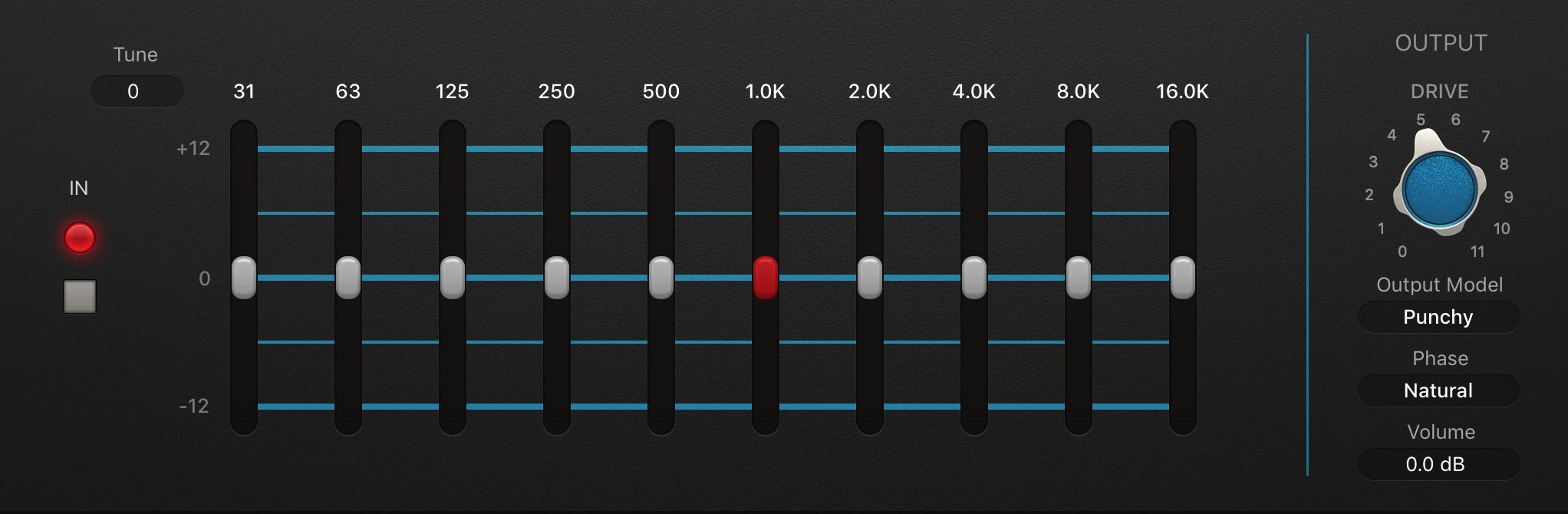
Logic Pro’s Graphic Equalizer digital emulation
Parametric equalizer - This is a specific type of equalizer that rather intuitively offers parametric controls for a more flexible approach to targeting frequencies. Parametric in this case referring to the various adjustable parameters to each filter available. This is nowadays the modern interface for most EQ plugins.

Parametric Equalizer featured above is Plugin Alliance’s Elysia MusEQ emulation
Filter slope (octave slope) - You may have heard filter slope or octave-slope when referencing the steepness of effect a filter might have. For example, a 12dB / oct slope for a low pass means that beyond the set threshold, the amplitude will be reduced by 12 decibels per octave as you progress higher in frequency. Likewise, a 24dB / oct filter will reduce beyond the threshold at 24 decibels per octave. These octave slopes are generally referring to high and low pass or shelving filters.
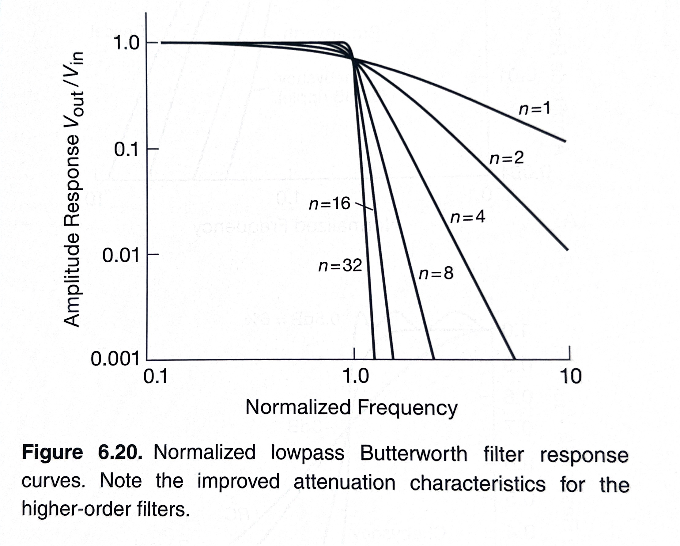
A butterworth filter is commonly found in audio circuits. This chart demonstrates various “poles” indicating the steepness in amplitude drop-off.
Image taken from The Art of Electronics - Horowitz & Hill
Quality factor (Q) - As touched on briefly in the section above, quality factor or “Q” on an equalizer refers to the specific filter’s resonance and bandwidth of effect. The “Q” parameter is common in most modern EQs, with filter types such as bell or notch, where the width of the filter can be adjusted from a very broad bandwidth to an extremely narrow set of frequencies you wish to pin point. The Q-factor functions somewhat similar to slope, in that it can adjust the steepness of the filter nearest the threshold, where lower “Q” means a wider transition of effect with low resonance. The reverse being high “Q” having a much steeper transition and potentially introducing a resonance peak at the threshold. This resonance peak may also bring about an unwanted “ringing” effect to your signal.

Quality factor controls for each of the filters featured on Plugin Alliance’s AMEK 200 inspired by GML 8200 EQ.
Poles - With regard to audio equalization, a “pole” refers to the point at which a proportional change in power begins to take place. “In one octave (as in music, one octave is twice the frequency) the output amplitude will drop to half, or -6dB…” as referenced with a simple RC [resistor | capacitor] filter. In physical circuits, having multiple RC sections leads to stronger reduction. You may be familiar with seeing 12dB, 18dD, 24dB, or more. When referencing these same filter slopes we might also say “three-pole filter” when using an 18dB slope, or a “filter with three RC sections (or one that behaves like one) p.52 Horowitz.”

SoundToys Filter Freak 2 - Each filter with an adjustable number of poles to determine the filters slope.
Phase / Phase rotation - This is a rather advanced topic, but crucial to effective decision making when it comes to equalizing. It’s the hard math in calculating the phase rotation of the signal you’re affecting. For example, if you were to duplicate your audio signal and flip the phase of the duplicate, the output of the summed signals would be effectively reduced to silence, as all positive peaks would be met with a reciprocal negative peak of the same power (phase cancellation).
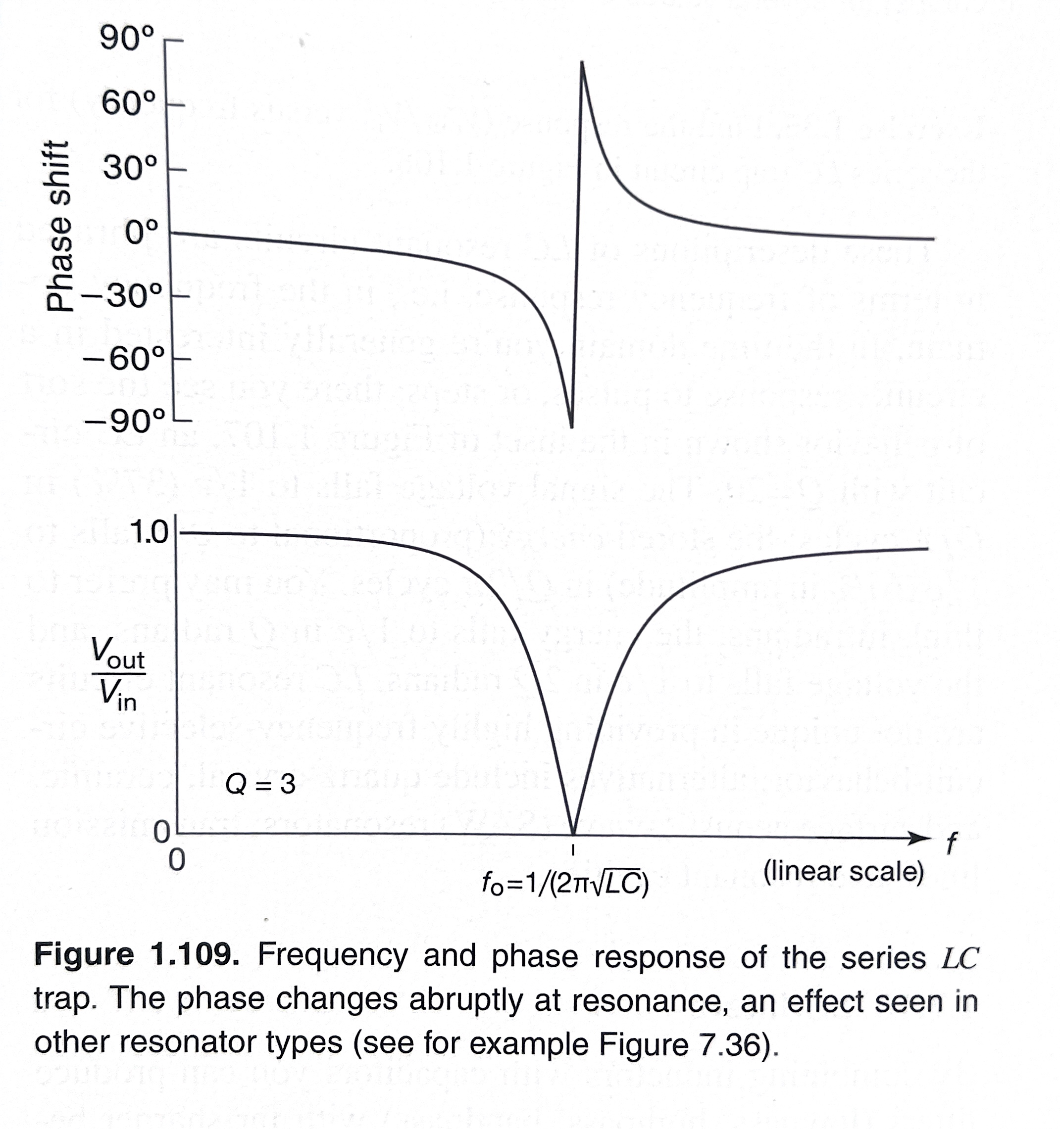
Phase shift of a notch filter (LC trap). image taken from The Art of Electronics - Horowitz & Hill
It’s easier however to understand with a simple sine wave, whereby adjusting the phase changes the timing of that particular cycle. It becomes complicated as you introduce multiple frequencies creating a complex waveform, and adjusting the phase of the overall output.
What if you were to return to the initial experiment of two signals, each of opposite phase, with an output of silence, and now add a notch filter to one of the signals? While you could hear the expected difference near the threshold, you may also hear some bleed of the surrounding frequencies, as each filter technically introduces an amount of phase rotation when applying gain adjustments. It’s useful to note that the steeper the slope / q-factor applied, the more noticeable phase distortion occurs typically.
Series / Parallel - Typically this would refer to the routing ‘under the hood’ of your equalizer. While this isn’t generally necessary information for beginning to use an EQ, if you’re familiar with the concept of series or parallel with regard to signal flow, it can be helpful for handling phase issues. If for example, you are introducing multiple bell filters in series, the resulting signal will compound at each filter with minimal phasing, as one simply leads to the next. However, if your EQ allows for the use of parallel filtering, you are effectively separating bandwidths, filtering, and then summing the final signal. There are advantages and disadvantages to both, and both can be used effectively, as long as you know what you’re dealing with. Ultimately, use your ears.
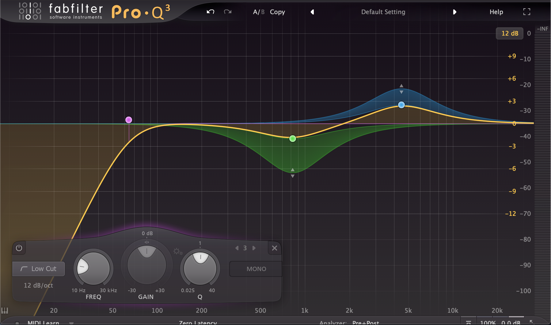
Brick-wall - Not to be confused with a “brick-wall limiter,” this filter type is mostly theoretical in the analog domain, as you can’t actually have an infinite reduction at a set threshold with time-based functions. You can get fairly close, however there will always be a discernible slope over a small spread of frequencies and quite a large amount of phase-distortion. This is not as much of a problem in the digital domain where clocking issues and latency can be accounted for, however it still won’t be a perfect reduction to unity at the threshold.

Fabfilter Pro Q3 - Brickwall filter
Filter types:
Low pass - A low pass will have a set threshold at a frequency (either fixed or tunable) where the signal is reduced in amplitude by a magnitude determined from the octave slope. In some modern cases, there may also be a “Q” parameter included to adjust the primary resonance at the set cutoff frequency.
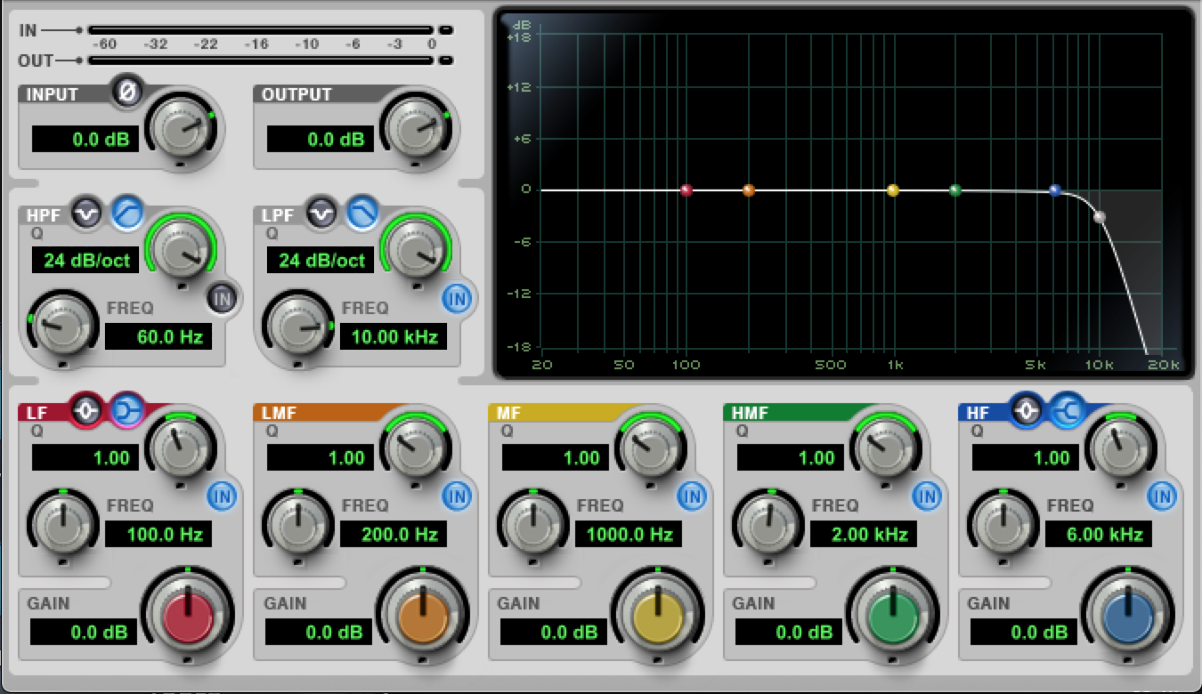
Avid EQ III - Low pass filter
High pass - Similar to a low pass, however reversed in the direction whereby frequencies are allowed to pass (high pass allows high frequencies). It will have all of the same parameters available to the low pass typically.

Avid EQ III - High pass filter
Bandpass - A bandpass is usually a tunable filter that allows you to filter out everything above and below a specific bandwidth (the signal within the bandpass sometimes referred to as the “passband”). There may be a few parameters offered with a typical bandpass, from oct-slope or “poles” as well as Q-factor. The slope will of course dictate how sharply the gain is reduced on both the upper and lower cutoff — in some instances the parameter poles will refer to how sharply the filter reduces on each side of the cutoff. However, the Q-factor (resonance in this case) is really what sets the tonality and bandwidth of this filter, as a steeper slope can begin to add a ring to your signal if the amplitude is affected heavily enough.

Fabfilter Pro Q3 - Bandpass filter
High Shelf - This filter is typically tunable (in some older cases limited to a bandwidth in the upper frequency range). Similar to high and low pass filters, there are both octave slope and Q-factor parameters, with an added gain parameter as well. The slope parameter functions somewhat differently, as the frequencies above the cutoff are not reduced completely. They are instead boosted or reduced to the amount set by the gain parameter. While incredibly useful filters, they can add unwanted phase distortion if the slope adjustment is too steep. You can in these cases use the Q-amount to ease into the cutoff frequency.

Waves Renaissance EQ 6 - High shelf filter
Low Shelf - Similar to a high shelf, however reversed in the direction the filter is aimed at shelving. It will have all of the same parameters available to the high shelf.

Waves Renaissance EQ 6 - Low shelf filter
Bell - A bell filter is probably one of the more common types in modern EQ’s due to its versatility for both precision and broad bandwidth adjustments. Historically these would have been set at a particular frequency [non-tunable], where adjusting the Q would allow for a less noticeable or softer change to your signal. You may also see some later versions with several tunable bell filters centered on a wide bandwidth. These later versions, while tunable to a certain degree, are limited to their set bandwidth [separated by sections — think low, mid, high]. Finally, with the most modern use cases in digital plugins, you have free range to tune and adjust wherever, compounding multiple filters centered at the same frequency if you so wish. This filter typically has a gain control, a frequency control, Q-factor, as well as octave slope.

Avid EQ III - Bell filter
Notch / Band Reject - This filter type is heavily used in sound system equalization for removing feedback resonances occurring within a space. They can also be used within a mix session to locate and remove problem frequencies, or for use creatively. As they typically cause a sharp reduction at very narrow bandwidths (notch filter) they also introduce an amount of phasing near the centered frequency. Similar to a majority of the previously mentioned filter types, the standard controls offered are frequency selection, Q-factor control, and slope or octave controls. There isn’t a gain control for this filter type, as the centered frequency is effectively reduced to infinity. With the octave and Q factor adjustments, you may also fashion yourself a band reject filter, omitting a much larger bandwidth from your signal.
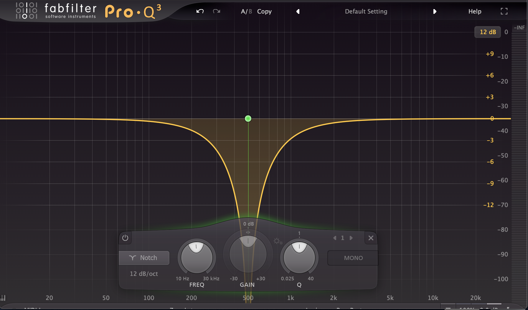
Fabfilter Pro Q3 - Notch filter
Allpass - The enigma of filter types for new engineers and producers, this filter can be quite a handy tool for dealing with phase issues. It does not function the same as previously mentioned filter types, where usually the goal is to alter the gain of a select frequency or bandwidth. Instead, it alters the phase of the signal by introducing a time-based adjustment across a set bandwidth. This “time displacement accomplished by an allpass filter is specified by its phase response. Allpass filters are used in circuit design to perform various frequency-dependent time-alignment or time-displacement functions [UA].” That’s a lot to digest… One example of an effective use case would be to alter the phase of the sub frequencies to help them sit within your mix more clearly. The only similar controls of an allpass filter from the previously mentioned filter types would be frequency selection, and perhaps any bandwidth adjustments. Think mono-compatibility when reaching for this device.
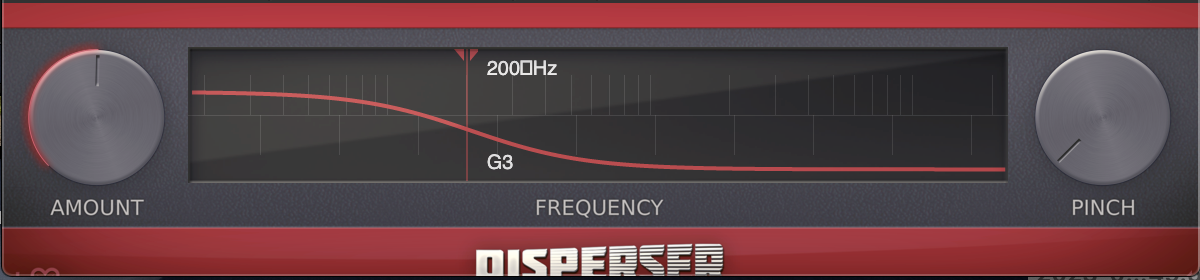
Kilohearts Disperser - Allpass filter
Baxandall Shelving - This type of filtering was made popular back in the 1950s by Peter Baxandall. It is a very subtle shelving slope introduced to boost gain in a less noticeable, or more pleasing manner. Effective on mix-buses or mastering chains, these subtle adjustments in gain have a low phase distortion effect on your signal.

Plugin Alliance’s emulation of the Dangerous Bax EQ - Baxandall type Equalizer
Pultec Style - This filter type you may hear thrown around in plugin emulation form, however it was made popular by the company, Pulse Technique’s “Pultec EQP-1 Program Equalizer.” It features a resonance attenuation just before boosting to a shelving filter. This subtle difference is an effective way to make the shelving boost appear more prominent to your ear.

Waves PuigTec EP1A modeled after the original Pulse Techniques - Pultec EP1A
Dynamic - These are the latest and fancy new additions to modern equalizer plugins. These Eqs typically allow certain filter shapes to have real-time gain adjustments that analyze your signal and reduce or boost at a set threshold. Similar settings in appearance to a compressor, however there isn’t a ratio setting and you aren’t actually compressing anything. Think of it as a fast reacting gain automation to a specific resonance frequency.
Fabfilter Pro Q3 - Dynamic EQ
Hardware Equalizers & Emulations
While I’ve touched on a few “filter types” above that were introduced through hardware units, it is far from the scope of this article to mention all of the numerous companies that have had a hand in advancing audio equalizers. Instead, I will mention a few reputable companies that are still around today, and have had great influence on the hardware emulation front. Hopefully to give you a place to start looking, as this rabbit hole is quite deep.
These images are included for demonstration purposes only, and are not an endorsement.

Neve - Formed by Rupert Neve in 1961, this company has been a mainstay of the audio engineering world. From full-fledged consoles, to rack mount hardware, Neve has been a pioneer for many companies to follow. Joining with AMS in 1990, they continue to manufacture anything from individual units to consoles solely designed for film post-production. You’ve more than likely come across an EQ plugin at this point that aims to emulate the style and sound of a Neve console EQ.
Solid State Logic [SSL] - If you’ve been around any recording studios featuring analog gear, you might have come across or heard of an SSL console. SSL was formed in 1969 by Colin Sanders, who had originally made switching systems for pipe organs. Throughout the 70’s he experimented, creating both the series A and B consoles, but it wasn’t until the 4000 E series in 1979 that the company broke through and changed the recording industry. There is a definite “sound” to two of the EQ’s associated with the later consoles — the brown and black EQs. To this day these consoles are still in use, and have many plugin emulations as well.

Brainworx SSL 4000 E channel strip emulation.
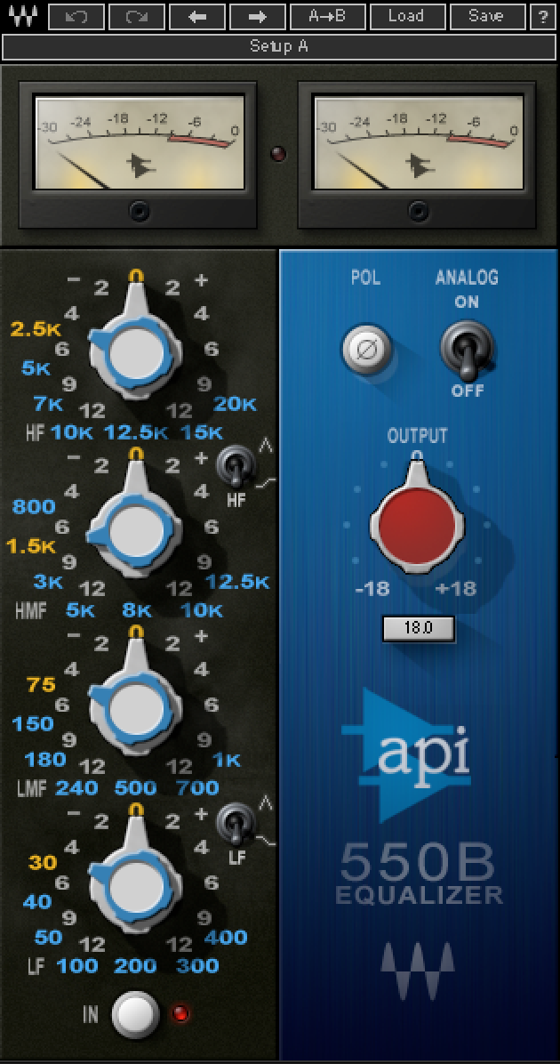
API - Automated Processes Incorporated, was formed in the late 60s, similarly to the previous two companies mentioned, by building a console. API has had contributions across the board with circuitry advancements, as well as the integration of digital total-recall systems as a very early predecessor to our current digital console workflows. API also manufactures rack mount units and likewise has many digital emulations of their hardware on the market.
Maag Audio - This company features mostly rack-mount units, but is famous for introducing the “air-band” to its EQs. The air-band is “a high-frequency shelving filter. But unlike most shelves, the corner frequency stretches beyond the audible range.” This might lend to the psychoacoustics or clarity of the sound, as it aims to lend a low phase distortion gain adjustment. As mentioned by Cliff Maag, “in picking the frequencies and Qs there was one goal in mind: No phase-shift. This lack of phase-shift determined the frequencies and Qs, which happened to create a big bottom end EQ that many users count on and have come to love…” You can’t miss the bright blue color that comes standard on all of their units.

Plugin Alliance Maag EQ4 emulation
Advent of Digital Plugins
If you’re producing or mixing for film or music, there’s a probability approaching one hundred percent that you have used an EQ plugin — It’s 2023, let’s be real. The current form of this device has become so incredibly flexible that it blurs the lines on some of these concepts, with the most advanced forms of these plugins offering dynamic controls [frequency specific reactive gain controls such as Fabfilter Pro Q3 or Sonible Smart EQ3). But, before going into some of the latest forms of these EQs, as well as discussing their advantages or disadvantages, I’d like to first explain the framework and limitations they operate within — your computer.
With the advent of personal computers, protocols were established for how audio data would be stored and read. While understanding this functionality can be helpful for troubleshooting errors that might arise within your signal, it is generally helpful information when applied to standard practice for handling audio files. You’ve no doubt had to set your DAW’s settings to a specific sample rate or bit depth, as well as the file format to ultimately export in. These settings will of course have an affect on the ways your tools (EQs, Compressors, etc.) operate, as well as the math applied under the hood. While these CPU processes are automated, it’s usually worth noting that larger file size likely implies a heavier processing power needed to accomplish the task at hand.
To understand sample rate and bit depth a little clearer, let’s imagine for a second how a computer stores audio information as bits. These bits within this virtual space could be pictured as stacked columns and rows of empty cubes that will hold a small portion of data about your signal as it passes through. The number of cubes in each row and column here are determined by the set sample rate and bit depth. For simplicity, we can imagine a clean sine wave function passing through this lattice structure of empty cubes — I find using a 3D representation helpful as you’re considering phase rotation within a stereo field, as well as bit depth, the value determining the scale of your signal’s dynamics. Because audio signals are a function of time, your computer will clock these values at this specified rate (48,000 samples per second in this example). You can further imagine this sine wave passing through these columns and rows of stacked empty cubes — each cube holding a freeze frame of the signal, determining it’s cycle or phase rotation, as well as frequency information. When compiling all of this information in sequence, your computer is able to reproduce this sine wave accurately, and produce a signal through your speakers.
Eventually these values were standardized as sample rates of either 44.1kHz or 48kHz with a bit depth setting of either 16 to 24 for lossless audio formats, such as .WAV or AIFF. Of course there are higher resolution settings available, however, the ones I’ve mentioned are currently accepted delivery formats for broadcast and streaming. “The slightly unusual sampling rate of 44.1kHz per channel adopted for the compact disc [CD] was derived from conventions already developed for the digital coding of video signals [Manning].” The reasoning of this convention has to do in two parts with the audible range of human hearing, [20Hz to 20kHz] and the processing rate to determine the fidelity of a given signal within a computer. Fidelity here referring to the retention of the most information as possible while reproducing a digital audio signal. To convey the full range of human hearing in detail, your computer must be able to process information by at least twice the highest frequency component present within the waveform [Manning].” This is due in part to the Nyquist Theorem, identified by Harry Nyquist in 1928. So, with the upper limit of human hearing reaching around 20kHz we would need a sample rate of twice that to accomplish an accurate representation of a signal.
(Why then did we land with sample rates higher than 40kHz. One reason has to do with something called aliasing — a type of unpleasant digital distortion. This occurs when the upper frequencies beyond the human register of hearing are folded back into your signal, causing unwanted harmonics. With an expanded sampling range beyond the Nyquist frequency, your computer’s digital converters are able to apply low pass filters to help reduce these occurrences. Further discussion of this topic is unfortunately beyond the scope of this article. If you wish to dive further, I suggest you check out “Electronic and Computer Music by Peter Manning.)
You might be wondering at this point, how does any of this relate to equalizer plugins? Cue the entrance of the bilinear transform… No you don’t need to know this math to understand or operate a plugin equalizer, but it is one of the few ways used to get an accurate digital emulation of a piece of analog hardware. Without boring you on the nuance of this process, it does have some implications for signal processing within an EQ. As the frequency affected approaches half the sampling rate, the type of filter used can cause what is called “cramping.” This undesirable effect occurs as the bilinear transform requires the signal amplitude to be at unity (zero) at the Nyquist frequency. This implies that certain filter types, such as a bell filter which has symmetrical effect above and below the centered frequency, would be distorted in the upper frequency. Modern plugins have mostly dealt with this problem by introducing internal oversampling, but it is worth checking your plugins manual, or perhaps utilizing an instance of plugin doctor to view how your EQ is affecting your signal (both in terms of gain as well as phase). While this is mostly an issue for mixing and mastering engineers to be aware of, it is useful information for producers as well — Especially when reaching for some random EQ that promises to fix all your problems.
Conclusion
I think some of the best advice I’ve received throughout the years is to find the tools that work for you and get comfortable with them. You don’t need to know every EQ, but it is important to understand how each of your tools are affecting the sound you’re hearing. While in most cases your stock plugins can take care of problem resonances or general rebalancing, there are of course professional third party digital options that offer flexibility only found in the digital domain. It’s hard not to impart your bias for the tools you swear by, and in this case it will come of no surprise to some that my recommendation for a swiss-army-knife type EQ is FabFilter’s Pro Q3. I don’t think I need to discuss this particular EQ further as this isn’t a sponsored message, but this plugin can handle most filtration issues you come across. My suggestion would be to start there, and branch out into companies like UAD, Slate, or Waves, to name just a few. Each will have their own set of standard EQ plugins as well as hardware emulations.
With a final word to equalizers, there is generally no perfect way to accomplish your goal, but rather a myriad of options to get you closer to your intended result. With each equalizer and/or decision leading to its own set of implications. If anything, hopefully this article gives you a better understanding of the process of equalization so that you might impart a more discerning taste when reaching for a particular EQ.
The further analysis of the latest forms of EQ plugins will probably have to wait until machine learning and AI have properly integrated into general use cases. Some of the most interesting EQs at the time of writing this, come from a company called Sonible — Their latest units allowing you to equalize reverb out of your signal, affect the transients of specific bandwidths, or even rebalance an entire instrument group… Some real dark magic if you ask me. As always though, use your ears, and remember your DAW’s stock plugins work just fine in most occasions.
References
All About Audio Equalization: Solutions and Frontiers, Vesa Välimäki and Joshua D. Reiss. MDPI, Applied Sciences Review. P. 2 section 2 (History of Audio Equalization).
Bohn, D.A. Operator adjustable equalizers: An overview. In Proceedings of the Audio Engineering Society 6th International Conference on Sound Reinforcement, Nashville, Tennessee, 5–8 May 1988; pp. 369–381.
Electronic and Computer Music - Peter Manning, p. 50 / 51 (filters), 246 (frequency & amplitude / transmission), 252 (high & low pass filters in digital to analog converters & vice versa), 256 / 257 (data register - sample rate and bit depth)
The Art of Electronics - Paul Horowitz & Winfield Hill, Third Edition, p. 14-15 (decibel readouts) 40 - 55 (Basic filter types), 391 - 405 (filter types - cont.), 406 - 422 (active filters), 310 (Op-amps and audio level distortion) 1109 (LC Butterfield Filters)
UA audio — Berners, D. (n.d.). Allpass Filters. Retrieved January 25, 2023, from https://www.uaudio.com/blog/allpass-filters/
Mäag Audio — Maag Audio History. Mäag, C. (n.d.). Retrieved February 22, 2023, from https://maag.audio/about/
Neve Audio — Neve History. Neve, R. (n.d.). Retrieved February 24, 2023, from https://www.ams-neve.com/our-story/neve-history/
Solid State Logic — Our History. Sanders, C. (n.d.). Retrieved February 24, 2023, from https://www.solidstatelogic.com/our-history
API Audio — About [page]. Retrieved February 24, 2023, from https://www.apiaudio.com/about.php
AT&T. The Historical Brands of AT&T. Retrieved February 25, 2023