In This Article
What is compression and how does it affect my audio?
There are a million posts from reputable sources on what compression is, what types of compressors there are, the history of compressors, and famous compressor units. Typically the authors of these articles aim for one of two sides, one being for the reader seeking best “use-case” information, and the second being a more technical writing of the science and math involved. Usually the latter is written with no remorse for a reader’s lack of knowledge on the subject and can be incredibly daunting to sift through for any useful information for their purposes.
I hope this reading helps to bridge that gap by further explaining some of the terminology used by electrical engineers. That way, you might be able to read through some of the technical jargon and at least get the gist of what the author might be stating. While I will touch on many of the aspects listed above, this is to offer a viewpoint on signal processing and how audio compression as a non-linear process can be utilized to its fullest. Full disclosure, I am an audio engineer — not an electrical engineer — but I’ve worked with these tools nearly a decade and hope to share what I’ve learned along the way.
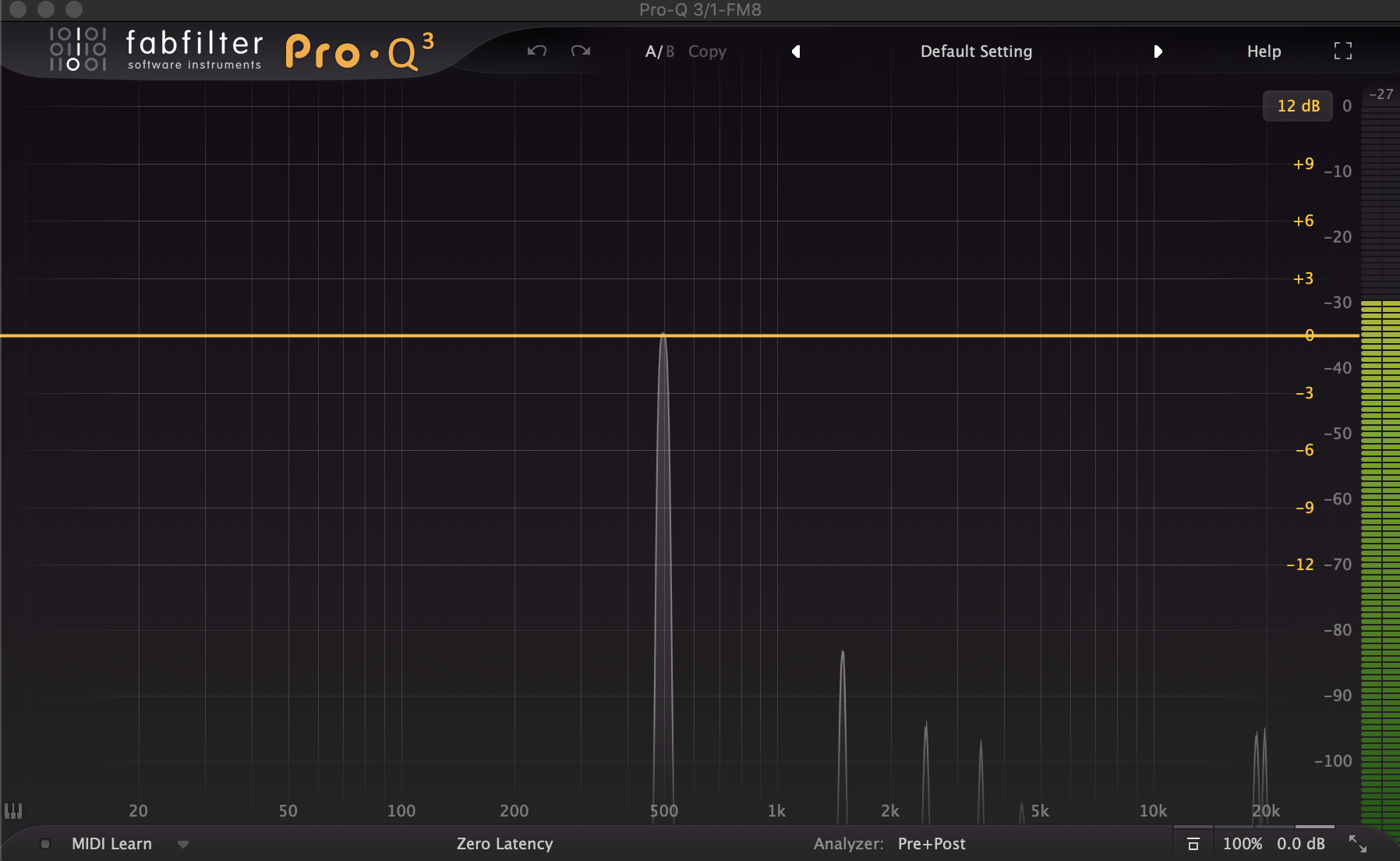
To start, compression is a non-linear function that applies an amount of signal compression, ultimately changing the overall signal (waveform) to whatever specifications have been dialed into the compressor. The “non-linear” aspect here being that it isn’t simply turning down your signal, but rather, altering the waveform through a set of parameters determined by the user. There are several different attributes of every compressor that we will get to in just a second, but first let’s talk about what non-linear means for someone who doesn’t quite have an idea of this concept in terms of audio. Say for example we’re using a pure sine wave. If you’ve ever used a parametric equalizer (similar to ones in DAWs like Ableton and Logic, or plugins such as FabFilter ProQ — ones with added visualizers specifically) You would see a peak at the frequency and amplitude the sine wave is set to from whatever source is generating your signal. If your sine wave is as close to pure as possible, you won’t have much of a clear view of upper or lower harmonics, but instead a lone peak at the set frequency.

Parametric EQ FabFilter Pro Q3 showing a sign wave near 500Hz
To take an exaggerated approach, set your compressor to the highest ratio possible, and your threshold pulled entirely down. You should have close to, if not an entirely silent signal (depending on what settings your compressor allows for). This is because your compressor has completely reduced the dynamics of your signal to zero (or close to it). By re-amplifying the signal with make-up gain we can bring up the signal with its harmonics introduced. Once the signal is changed through compression we can view through this parametric equalizer where the harmonics have become more prominent. When the signal is forced to interact with this threshold it changes the original waveform by compressing the most dynamic features, with an amount of saturation occurring to the most dynamic peaks. Depending on the material, it generally acts by bringing the resonant peak down, closer in amplitude to its upper harmonic material. If you were to look at a zoomed in waveform within your DAW at the sine wave before and after compression has been applied, you would be able to see the effect on your signal as modulations to the shape of the sine wave (below is an extreme example).
Parametric EQ showing a sine wave near 500Hz with harmonic saturation from compression.
What is important to remember though is that this view through a parametric equalizer is a two-dimensional snapshot of a continuous process (limited by the refresh rate of your visualizer and CPU’s processing power). In other words, sound waves move continuously, completing multiple cycles per second, and the signal can change over time with different frequencies and amplitudes presenting simultaneously.
Without having to go down a nerdy science rabbit hole, it is important to remember sound waves are not some static process, but have variable changes throughout time. These EQ visualizers, while a nifty tool to indicate what frequencies are present with a limited scope, aren’t giving you the whole picture. Use it only as supplemental to what your ears tell you, especially when it comes down to what your compressor is doing to your signal.
In an attempt to demystify the process of compression, let’s talk generally about their function as a physical circuit (again trying to keep it within general terms). To start we have to briefly remember that this was a technical process invented to attenuate (reduce in value) a desired signal and there was in fact math and electrical engineering involved. You will however have to make some concessions, and at least learn a few terms and concepts to fully understand compression overall. These aspects carry over into different discussions of audio engineering and can be helpful bits of knowledge moving forward.
Types of Compressors
For quick context:
Below I go over some common types of compressors used and some of the famous versions of these you might come into contact with. This is generally helpful information as it will give you a head start on how/when to use one of these compressors with your material. It is a bit more technical as I attempt to cover the different circuit types in each compressor with a general summarization of their effect. If you don’t really care about this information you can jump down to the “Use-case” section where I go into the effects of each parameter on a given compressor.
Delta-Mu (Variable-mu)
Some of the earliest compressors were called Delta-Mu compressors, (Greek terms “Delta” referring to change, and “Mu” referring to a measurement or in this particular case, gain) or “Variable-Mu” as coined by manufacturer Manley for their versions of this type of compressor. While the circuitry can be somewhat different from each unit/manufacturer, the overall process of compression was more or less the same. What these early compressor circuits utilized was a series of vacuum tubes ran in parallel. These two channels of tubes (gain reduction circuits) receive a voltage which is referred to as its variable bias. The first channel receives an unchanged version of the original audio, while the second receives a reversed polarity copy — polarity referring to the orientation of the positive/negative peaks within a cycle of the waveform.
As you adjust the dials to whatever settings you desire, the tubes would apply gain reduction to your signal in accordance to your settings (here’s where a lot of the math and electrical engineering occurs that I conveniently gloss over). At the end of the chain, the amount of bias introduced by the vacuum tubes running in parallel is cancelled (subtracted) out through the transformer output and you’re left with the remaining compressed audio signal.
In fact, the more you increase the gain of the audio signal, the more compression is applied and eventually heavier amounts of saturation occur as the transient peaks of your signal come up against the compressor’s threshold. Without having to dissect the schematics of old compressors, that’s a good start. It’s probably enough information to know that your audio passes through electronic components (in this case tubes) which are ultimately the pieces that impart an amount of character, tone, and of course compression to your signal.
Some examples of Variable-Mu compressors would be the Manley Vari-Mu, Fairchild 660 and 670, and Chandler Limited RS124. Later came circuit types such as VCA, Optical, and FET compressors. Each of these apply compression through different processes, giving varying types of coloration and saturation to your signal.
VCA compressors (Voltage-Controlled-Amplifiers)
VCA compressors might be some of the most common. They typically have all of the settings users have become familiar with when using compressors: attack and release, threshold, ratio, and knee. While I won’t be able to break down the schematic as much as the Delta-mu compressors, I’ll try and explain it as best as possible. Also, similarly there might be some variance to each unit, e.g. where in the circuit’s routing the compression is applied, but again they more or less function the same — at least in a “use-case.” Basically, as Voltage Control Amplifier might imply, it supplies a voltage to an “amplifier,” which determines an amount the compressor will “attenuate.” It’s important to note that VCAs are not limited to use only with compressors, and if you’re just starting out you might see the label [VCA] with a number of different units. This is because it is a circuit type utilized to send an amount of information through voltage, which can then be interpreted for a modified outcome. In the case of a VCA compressor, you’re sending the attack/release, threshold, ratio, and possibly knee settings (if available on your particular unit) from the “rectifier” circuit which converts AC - alternating current, to DC - direct current. These settings you’ve dialed in tell the circuit how to apply compression or attenuate your signal.
VCA compressors offer a much more clinical control over your sound and are usually referred to as more “transparent” sounding. Some examples of VCA compressor units range from the DBX 160, the SSL E and G-series, and the API 2500.
Optical Compressors
Optical compressors are different in that they convert their audio signal into light using an optical photocell array. This light signal varies in brightness with the amplitude of the audio signal, which is then received by a light sensor or photoresistor, which changes its impedance based on how bright the light is. This interpreted information determines how much gain reduction should be applied to the audio signal.
(In the early years of optical compressors, the light source utilized was a filament lamp or other electroluminescent device. LED lights replaced these earlier versions as they were much faster, however they required stronger voltage to work).
A famous version of this compressor you might have heard of is the Teltronix LA-2A engineered by Jim Lawrence (founder of Teltronix), which uses a T4 optical attenuator (<- photocell). These compressors counterintuitively react slower and have been known to have a “musical” quality to them. Interestingly, these compressors are also frequency-dependent, meaning the ratio of compression applied can vary across the frequency spectrum of your signal, applying more compression as the amplitude of one frequency range increases over another.
The release function is also pretty slow; this has to do with the physics of the photocell attenuator. The best way I could describe it is when you turn on and off a light in your house, if you catch a glimpse of the bulb as it’s shut off it doesn’t actually lose its light instantaneously, but instead cools quickly dissipating the heat of the coil. Obviously these compressors aren’t using incandescent bulbs, but the physics are still true. The longer you supply current or the stronger the amperage, the more heat will be introduced into the system, and the longer it will take to dissipate, or in this case release. Some examples of Optical compressors are the (as mentioned) LA-2A, the LA-3A, and the Tube-Tech CL-1B.
Fet Compressors (Field Effect Transistors)
Finally there are FET compressors. These compressors are some of the most defined in terms of sound quality, and in fact are used in some instances with the compression aspect turned off, using it solely as a preamp for the sound quality of its input/output transformers along with the transistor circuitry. It is also the most complicated compressor circuitry (in my opinion), and where I found the most difficulty trying to break it down into more understandable terms — I had to break out an electronics textbook as well as peer through the UREI 1176 manual to have a better understanding of how this thing works…and with only limited success.

A couple images from “The Art of Electronics,” by Paul Horowitz, to give you an idea of how complex the material is when it comes down to the math applied within the circuit.
But, here goes nothing: A FET (field effect transistor) as the name might suggest conducts via an electric field. It has to do with the actual material of the circuit board and the components used to drive the signal. Basically its benefits come from solid-state electronics and negative feedback circuitry granting its ability to maintain a high impedance that isn’t necessarily dependent on high input.
That might sound like a bunch of big words with little meaning if you’re unfamiliar with the subject.
Ultimately, the process of compression is self-contained within this circuit type, where the output of the audio signal is able to send feedback to the compression process to further determine how it is attenuated. At face value this doesn’t make any sense, considering the output of the compressed signal determines the attenuation of its input, but one would probably need a better understanding of the physics at this level for it to seem at all intuitive. At this point historically speaking we’re on the cusp of this technology being utilized for advanced computation, so if you also find it complicated, that’s okay. All that said, I’ll leave you with this: FET compressors impart their tone and harmonics through their specific array of components, namely their transformers and transistors.
The most famous FET compressor is probably the UREI 1176 (Universal Audio) as mentioned above, and is still widely used on a number of major records to this day. As mentioned, these compressors are famous for their incredibly fast attack and release response times. They were an improvement to the optical and Variable-mu compressors lacking on this front.
Because of these specs, they were referred to and used more commonly as peak limiters, as they were able to control transients better than say an LA-2A with a slower attack time. In fact, the slowest attack times of the 1176 are in most instances faster than the fastest attack setting of a Variable-mu compressor — 20 to 800 microseconds according to the manual. That’s right — microseconds, not milliseconds. Definitely useful information when you’re deciding what to use for your signal processing. Other examples of FET compressors are Chandler Limited Germanium Compressor, and Daking FET III.
Compression vs. Limiting
Okay, so we’ve covered several of the main types of audio compressors utilized to this day, and in fact there are still more, although less common types, like diode bridge compressor/limiters by Rupert Neve or the obvious digital compressor. The ones I’ve covered hopefully help to give a better understanding of each of their internal circuitries and how they react to audio signals. While I spoke more generally towards the concept of compression, it’s probably important to recap on some of the peripheral concepts introduced in this discussion. Namely peak limiting vs. compression (with RMS metering), as well as saturation and types of clipping.
This area I think generates a lot of confusion for new engineers/producers, and rightfully so. There’s a lot of crossover conceptually of other processes that offer a more specific quality to your sound. You may have heard the terms saturation or clipping when discussing limiters and compressors. This is referring more specifically to your signal’s transient peaks coming into contact with the threshold of a compressor or limiter, and the process involved in shaping your waveform to a more leveled amplitude. This comes back to the concept being a non-linear process. As the compressor is engaged, it clamps the highest energy transients peaking beyond the threshold, and pushes them more inline with the quieter parts of your signal that remain below the threshold. This process is not a clean change in gain, meaning it does not retain the original shape of your waveform and in fact distorts it somewhat.
This amount of distortion can be referred to as saturation. While I could probably write an entirely separate article on distortion and saturation, it’s important for the discussion of compressors and limiters to have a general understanding of the effect.
In discussion, saturation is usually utilized to describe the warm tone or harmonic boost to your signal. As mentioned, it is the process of your waveform coming into contact with a threshold or ceiling that physically shapes your transient peaks. In the case of a compressor or limiter, it will interact with your transients as a function of the specific parameters you’ve set, and compress/limit accordingly. Because the difference between compressors and limiters is in the time domain, the shaping of the waveform is more drastic with one compared to the other.
If you guessed limiters as the more extreme, you are correct. Limiters are quite intuitively named for their ability to peak limit, and in the case of your audio signal, it is able to clamp down even within microseconds, acting seemingly instantaneously. This drastic shaping is sometimes referred to as clipping if applied heavily, as it literally clips off the peaks of your signal and you’re left with a “squared” waveform. You may in some cases find different settings on your compressor for soft clipping or hard clipping. This allows you to vary the amount of shaping to the waveform as well as introduce and amount of saturation or distortion to your sound. Each form of clipping has a very distinct sound quality, and if you’ve ever clipped your meters in your DAW, that too is a form of digital clipping (although an inadvisable technique to achieve clipping.)

An image of an uncompressed sine wave on the left, and a heavily clipped sine wave on the right, more closely resembling a square wave in appearance and tonality. Example made within Ableton 10.
Generally speaking, this is not usually what you’d aim to do with your sound and historically is described as very unpleasant. We are, however, living in a post-dubstep world, and if you peek under the hood of the audio engineering scene, the loudness wars are still very much taking place. These heavily compressed waveforms would then be turned back up to effectively squash the dynamic range of the program material. Just peruse the current top-40 charts and listen to the drums in comparison to vocals.
With technological advancements on a digital front, consumers have been able to utilize compression and limiting techniques that would normally be reserved for audio engineers within a studio. There are pros and cons to this obviously, but that’s a separate topic and ultimately it’s here to stay. So, you might as well know what you’re doing while using them, and know how and when to apply the effect with intent. Before getting into compression parameters, I wanted to wrap up with a couple points on headroom as you may have heard the term thrown around a lot. The process of compression and limiting is directly tied to the concept of headroom.
Maybe you’re starting out and you’re wondering where to set your kick and snare levels within your mix, or perhaps you’re told to “leave enough headroom for your mastering engineer.” You might be working on a film and you’re trying to consider the fact of whether your film will make your audience’s ears bleed from being too loud. These are all real world examples of considering headroom, and what isn’t mentioned is “how compressed is your program material already?”
The general assumption is if you leave enough headroom, then you’re fine, but this doesn’t fully take into consideration that you have a finite dynamic range. If everything is extremely compressed already, then any further levels of compression may ultimately change “the mix” for better or for worse. More importantly, if one track of your mix is incredibly compressed while another’s dynamic range is left untouched, that relationship (if within the same frequency range) cannot be changed by some mastering engineer’s magic.
Parameters
Below I go through a more technical usage of a compressor and how it can be utilized through a familiarization of some basic concepts. While my aim is to give you a better understanding and hopefully speed up your process of learning, you will ultimately need to spend time with each circuit type, passing numerous signals of varying frequency responses through them to really grasp the effects for yourself. First, let’s consider the various parameters available on a given compressor and then after we’ll discuss different “use-cases” for each.
Parameters you might find are:
Input/Output
Ratio
Threshold
Attack & Release
Knee
Peak / RMS settings
Make-up Gain
Look-ahead
Low/High Pass Filter
Side-Chain
Mix

To the Upper right are a couple examples of compressors displaying a mix of these parameters. Pictured above, the Empirical Labs Distressor (Analog Compressor) and below, FabFilter Pro-C2 (Software Compressor).
This may not be an exhaustive list, but should mostly cover what a typical compressor might have. Conversely, many will not have all of these parameters, and in some cases only have an input and output.
Input/Output
Pretty simple: input controls the gain of the incoming audio signal, while output controls the compressed audio’s output gain. If you’re working with an LA-2A you’ll only have these two knobs to control your signal, while the compression takes place directly from their relationship.
Ratio
If your compressor has ratio parameters this is to determine how drastically your compressor responds to the signal crossing the threshold. In most modern cases, there is a single ratio knob that can be turned from 1:1 (not compressing) to infinite in some cases, with anything over 10:1 being considered limiting. Your compressor’s ratio is directly tied to the threshold where for example if it were set at 4:1, for every 4 decibels of gain beyond the threshold, it would be reduced to 1 decibel over the threshold. Most limiters utilize infinite ratios and will heavily alter your signal if pressed hard. You may remember that I mentioned the UREI 1176 is a “peak limiter,” however this compressor has 4 separate ratio settings of 4:1, 8:1, 12:1, and 20:1 which you can choose individually, or press all at once for a healthy amount of compression.
Threshold
This is where the function of compression begins to take effect as your signal crosses beyond it. If your compressor has this function, you can determine the amount of dynamic range you’d like to reduce by setting this with consideration to your ratio.
Attack & Release
This determines the character of compression taking place. In most modern cases your attack and release are set in milliseconds, where the attack determines how quickly or slowly the compression takes effect, while the release determines how quickly or slowly the compression disengages. Depending on your compressor’s circuit, these functions can act more linearly or with a slight curve where the effect is gradually applied or released. It is also important to remember that these settings should be determined by your program material. If the compressor does not have enough time to release from one transient to the next, your signal will compound its compression and more heavily shape your waveform’s dynamics. Although the 1176 doesn’t have numbers to denote the attack and release settings, it’s good to know that the attack function is actually in microseconds rather than milliseconds. Most limiters will only have a release setting (brick wall limiters) as they take effect as soon as the signal reaches the threshold. There are rare occasions where your limiter might have an attack setting, like the FabFilter Pro L series, and this may seem confusing considering it is supposed to “limit” anything from passing beyond your set threshold. To my understanding, it is more of a determining factor of the shaping happening at the threshold, similar perhaps to the “knee” function.
Knee
This determines the linearity of your compression threshold. As mentioned above, some compressors allow you to determine how its function engages, where a soft knee means compression will more gradually begin, typically with a shape that resembles a logarithmic curve. A hard knee usually means the compression takes effect more closely (or exactly) where the attack and release parameters are set. With compressors like the LA-2A, the knee function is ingrained in the circuit itself and dynamically changes based on your signal coming into contact with the threshold — most notably with the release function.
Peak/Rms
This can refer to both the detection method as well as the metering type, where peak refers more so, to a discrete process of detection, while RMS is more of a continuous process. In general, peak limiting refers more to limiters and fast acting compressors, while RMS is a slower function of detection that works in response to the average loudness of your signal. Most compressors these days will come with at least one of these meters, whether it’s a visual pin meter quickly flipping from right to left in response to your signal’s gain reduction, or a digital readout in stacked bars denoting a number of reduced decibels. With peak limiters, it is tracking the decibels reduced in stricter terms, where transients that pass beyond your threshold by the amount your ratio is set to will be limited. This amount will be displayed on your peak limiter, so if it reads 3 decibels of gain reduction (GR), you’ve attenuated the transient by exactly that amount. With your compressor working in RMS mode, it’s a little different. You might recognize RMS or root mean square from past math classes as a tool to calculate the average amount of change within a continuous process. In our case with an audio signal, the concept is applied to the rate your waveform is compressed. The way it works is your compressor analyzes the average loudness of your signal over a short period of time and begins to apply compression more steadily for a more evened out leveling. In some cases, it might make sense to use one compressor focused on mild peak limiting, with another afterwards, that applies RMS compression to even out the tone. *coughs* 1176 followed by LA-2A.
Make-Up Gain
By increasing the make-up gain, you’re increasing the compressed signal back up closer to its original perceived loudness. The difference here between the makeup gain and output gain has to do with a mix knob, which I’ll explain in more detail in just a moment. It is important to know that if you attempt to raise your gain using the output rather than the makeup gain, and then dial back the mix knob from wet to dry, you could potentially have unwanted variations in the dynamic range of your signal. Makeup gain gets rid of this by putting the gain compensation in front of the Mix knob.
Look-ahead
This is a more modern process within digital compressors and limiters, and offers your unit the ability to “look ahead” at the signal before it hits its detection circuit. In the case of a limiter, this can help to make sure no transients sneak by the threshold. It will, however, affect the latency of your signal, so you’d want to be careful about adding too much look-ahead and potentially slowing down the placement of your audio in relation to other sounds within your project.
Low/High Pass Filter
If you’re familiar already with EQs, then this concept is pretty straightforward. While this can be found on some hardware units, as well as console channel strips, it is a way of altering the detection circuit for how and when the compression is applied. if you set your high pass filter to 100Hz, everything below will not be fed to the detection circuit (keep in mind this is probably a roll-off of 12db to 24db respectively — if using FabFilter you can change the curve). This means that, although the compression is affecting the entire signal, it will not react to the most dynamic portion of the waveform (in this instance). In some occasions, you might even be able to create an EQ curve to accentuate or lessen the focus of the compression on specific bandwidths of your signal.
Side-Chain
If you’re working in an electronic music genre you’re probably familiar with this process, as it has become a mainstay of the style. What side-chain does is allow your compressor to input an outside signal from another track or group of tracks, and then apply compression to the original signal based on this external signal. This might seem confusing at first, but basically it’s a matter of understanding the routing happening within the compressor. If your compressor is on a channel containing a synthesizer, and you have it paying attention to a kick on another channel, your synthesizer will “duck” or be compressed (by the parameters you’ve set) when it interprets the transient of a passing kick.
Mix
Finally we have mix. This is at the end of your plugins routing, just before output gain. It will have a knob or fader that determines the amount of “wet” or “dry” signal is passed through. With your mix knob set to 100% wet, your output signal would be sending out a 100% compressed signal. What this is actually doing is parallel mixing in a compressed signal with the dry signal, so if you dial it back to 50%, you’re effectively sending half of a dry signal through and half of a compressed signal. That may seem pretty obvious, but for clarity’s sake, we’ve come this far. The more you know.
Alright take a breather. We’ve gone through a lot of the technical jargon describing what a compressor is, types of compressor circuits, and what it does to your signal. Now to consider your program material (Referring to your signal more broadly, as the contents and platform of release might range from music, film, television broadcast, podcast, etc.) I will primarily focus on the platform of music, as compression takes on a more creative means within the art-form.
Use-Case
This is usually the portion that is left out in compression articles, which makes sense considering there are seemingly an infinite number of sounds you can pass through a compressor. Technically, it’s an art form, so you may decide to apply compression clinically in one scenario, while in another you destroy your audio’s dynamic range. What I will try and do is approach this from a couple modes of thinking, but they are in no way the only ways to approach each problem.
Say for example you have a snare. It probably resonates around 200Hz, or a kick somewhere around 100-110Hz, or a clap around 500-600 Hz. All of these sounds will generally have upper and lower harmonics and won’t appear on a frequency analyzer like a clean sine wave did in our earlier example. With that in mind, how would you go about deciding your settings for compression?
Here there are two main things to consider before you decide your settings, and it comes down to what your aim is for the outcome of your sound. Are you aiming to control your signal’s transients or accentuate or shape your signal? This can seem confusing, as you may have surmised you could in fact control AND accentuate your sound. One example of this might be to control or attenuate the lower frequency dynamic range of your kick, allowing you more headroom to turn the kick’s gain back up for more perceived loudness (Not saying you’d want to do this, but you could). This becomes further complicated by the fact that one sound in a particular frequency range may have a different effect on your overall track’s headroom than another, and this comes down to frequency wavelength.
So let’s nerd out for a second by talking about frequency and how wavelength can differ from one end of the spectrum to the other. You might know that the human range of hearing is approximately 20Hz to 20,000Hz, with most visual analyzers for audio displaying this range. You might also know the speed of sound is roughly 343 m/s at sea level and 20 degrees celsius. Before you get all freaked out, you don’t need to remember this. It is, however, helpful for understanding the next portion. We’re aware the speed of sound applies equally to all frequencies, but what we haven’t considered is the time it takes for one wavelength of a given frequency to propagate.
High-frequency wavelengths will take a shorter amount of time to complete a cycle as they are physically smaller, while sub frequencies will take much longer, relatively speaking. For example, a 50 Hz audio wavelength is roughly 22.5ft. That seems like an incredibly long wavelength, but at the speed of sound, it only takes milliseconds to complete — in this instance 20 milliseconds. On the higher frequency end, let’s say 10,000Hz, the wavelength is just barely over one inch (1.3in) and takes only .1 millisecond (or 100 microseconds). You might at this point be putting together the pieces of what I’m suggesting — a compressor’s attack and release settings are denoted in milliseconds (with the 1176 in microseconds). Below is a small table I’ve made as a cheat sheet.

Table of frequencies in Hz, and their relative times to propagate at base conditions (sea level and 20 degrees celsius). Useful if your aim is to have attack times set for specifically peak limiting.
These values might be helpful to consider if your aim is specifically to limit transients. It is important to note this guide isn’t going to be exactly correct every time, as it doesn’t take into account the amplitude, duration of the signal, or how complex your waveform is. It is at least a helpful guide for familiarizing yourself with frequency in Hz and what attack/release settings to begin with in order to limit frequency specific transients. I’m in no way advocating to rely on frequency analyzers to determine what compression settings you should use either, but knowing this information can help you internalize what you’re hearing with what you’re seeing and interacting with. In the long run, hopefully you’ll hear a sound and know where to start with your attack/release settings, and then adjust to taste.
Lastly, let’s talk about accentuating or shaping your sound. As we just discussed limiting the initial transient of a waveform, let’s take a step back to see the big picture — in this case one “beat” within a song. Why one beat you ask? Because we typically describe the tempo of a song in BPM or beats per minute. So for simplicity sake, let’s say we’re working with a song at 100BPM. One minute converted to milliseconds and divided into beats gives us 600ms per beat (if you’re making dance music 128BP = 468.75ms). Again continuing with simplicity let’s say it’s a track with a four-on-the-floor pattern and the kick on every down beat. If we were to compress our kick we would want to make sure that our compressor has enough time to release before the next kick transient hits in 600ms. Your kick is most likely not going to take up the entire 600ms, so let’s say it’s around 250ms (depending on genre your kick could be shorter to leave space for 808s). Now we want to accentuate the sound, so we aim to set our attack and release settings with consideration to the decay of the kick sample. To bring out the decay or tail of the sample we’ll want to have settings slow enough to allow the initial transient to pass, and long enough release that it doesn’t cause distortion or unwanted pumping (fast release times can cause a jump in gain [pumping effect] and if during the period of a low frequency waveform, possibly distort your signal). Once we have our settings we can dial in the desired makeup gain for added presence.
I don’t have specific timings to suggest here, because at this point it’s fairly dependent on the sample material. In almost all cases you probably won’t need to calculate the number of milliseconds per beat to know how to apply compression. This is however, a useful example for understanding how one beat within a measure of your track is broken into units that your compressor measures audio signals — milliseconds.
You probably won’t have as straightforward an example as used here and will have to adjust accordingly to complex rhythms or conflicting frequencies. Ultimately, the most important thing here is to use your ears. If it sounds good to you, then do it. There will always be a number of people that will jump at the chance to say you’re doing it wrong, but luckily purists usually aren’t tastemakers. Take the time to learn this tool, and how you can shape your sound for whatever platform you aim to release your content.
Now that you know a bit more about compression, I’ll leave you with this final note. YOU DO NOT NEED TO PUT IT ON EVERY CHANNEL.
SOURCES
Horowitz, Paul. The Art of Electronics, Third Edition. Winfield Hill, Roland Institute at Harvard. Cambridge University Press. 1980, 1989, 2015.
ArpJournal, UREI 1176 Manual, UA-LA-2A, UA-1176, VintageKing, SoundonSound, SoundAU, SoundAU_2, MobTown, 4SoundEngineers, iZotope, SoundBridge, Pulsar, electronic-tutorials, wired, jdbsound, who.int, sciencing, 1728, AudioHertz